The aim of a neutrino factory is to produce intense beams of neutrinos by trapping muons in a storage ring until they decay. Muons, having a half-life τ½~1.56μs, are not readily available in nature and must be produced earlier on in the accelerator system. The suggested way of doing this starts with a proton beam of several GeV and fires it at a target material, which emits pions (π+) that decay into the required muons (μ+) soon afterwards (τ½~26.0ns).
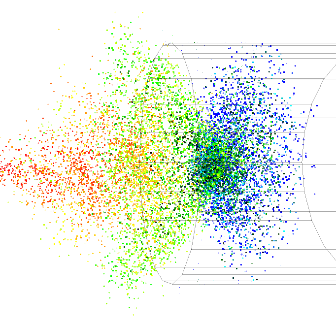
The main difficulty with this scheme is that the distribution of pions emitted from the source has an extremely large emittance: in the dataset used, 22% of the pions are actually going backwards in the lab frame (vz<0), so the emittance can hardly be calculated. This means that any simulation based on conventional assumptions about the beam's general direction and size are likely to be inappropriate. There are inevitably large losses associated with capturing this beam and focussing it into a form that could e.g. be accepted into a linac.
The decay of the pions into muons adds another unusual element to the system, as the other decay products are emitted at high speed and make significant changes to the original particle's mass and velocity. The pion half-life corresponds to 7.8 light-metres, so the decays happen on the same timescale as it takes the particles to travel through the first few magnets. This effect also makes simulation with a traditional tracking code potentially inaccurate.
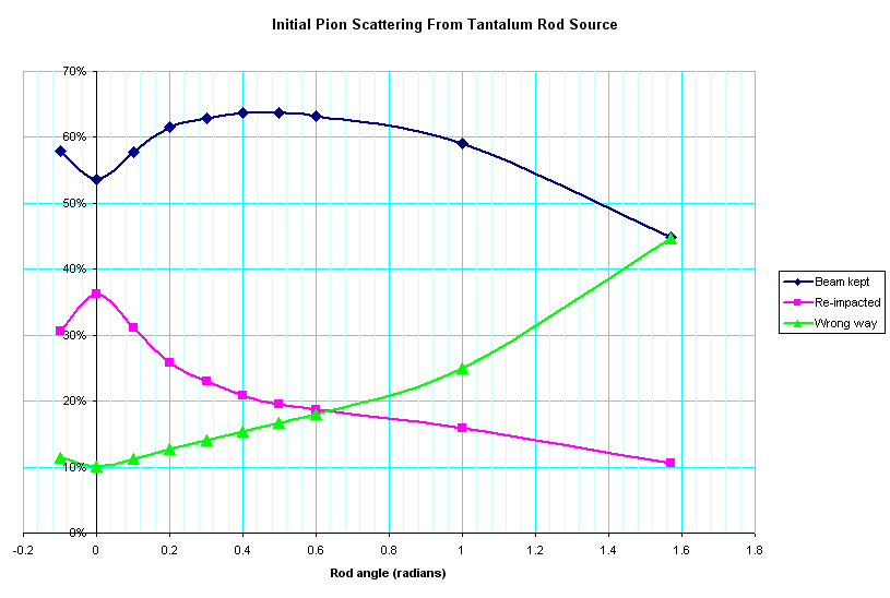
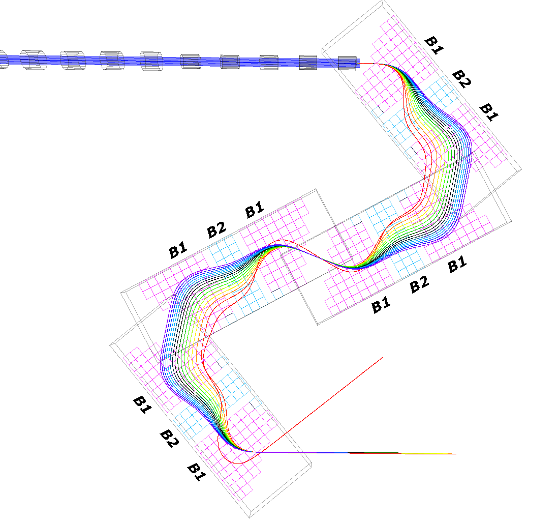
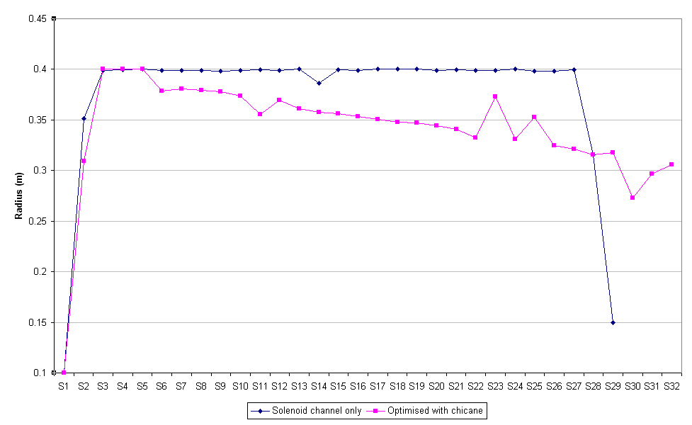
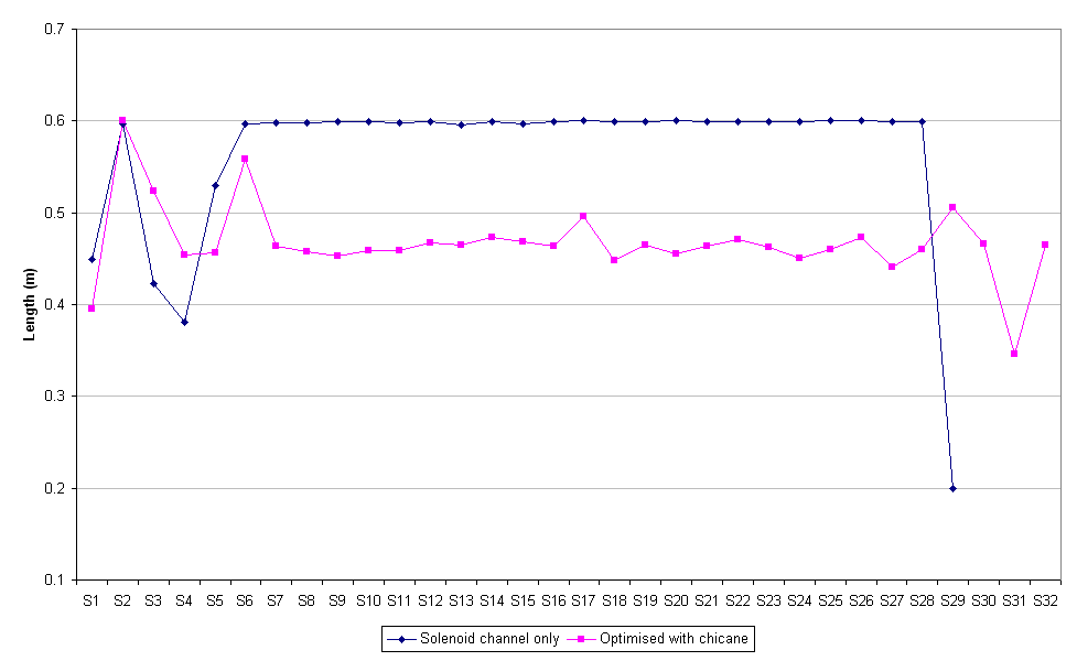
This report focuses on the proposed design in which the pion source is a tantalum rod (20cm long, 1cm in radius) being hit by a 2.2GeV proton pulse, assumed to have a Gaussian longitudinal bunch shape of RMS one nanosecond. The first component in the muon capture apparatus is a channel of transverse-focussing solenoids, the first of which encloses the rod (although the axis of the rod need not be parallel to the axis of the solenoid). The lack of longitudinal focussing means that the particles with larger vz will work their way to the front of the bunch, which will have spread out somewhat by the end of the channel. With this in mind, the next component is a 'chicane' of specially-designed bending magnets, in which the faster particles will go on paths further to the outside of two opposing bends in the accelerator.
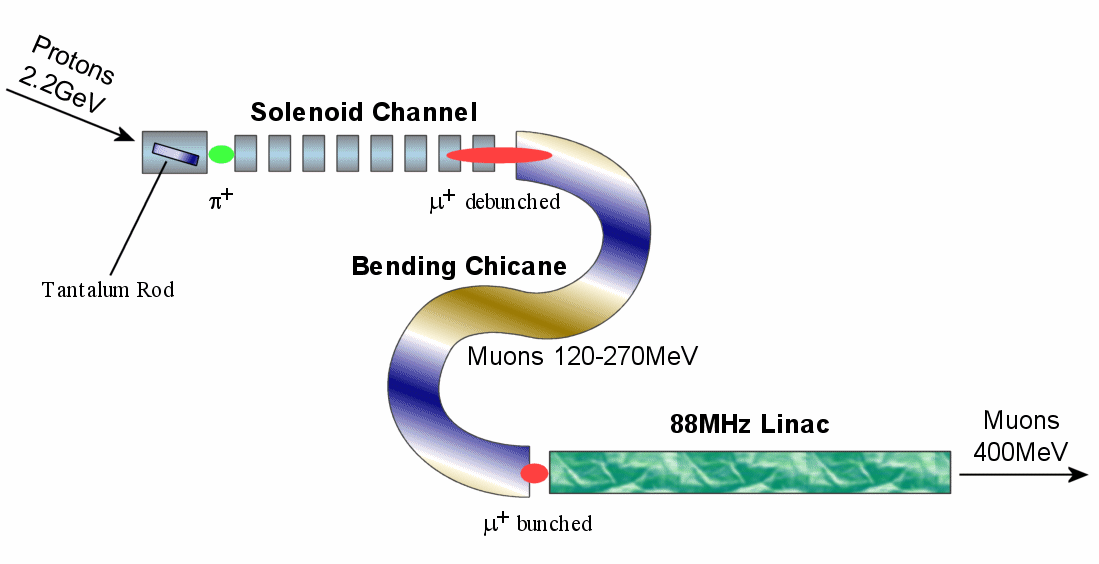 |
| Figure 1. Schematic of the RAL muon front end design. |
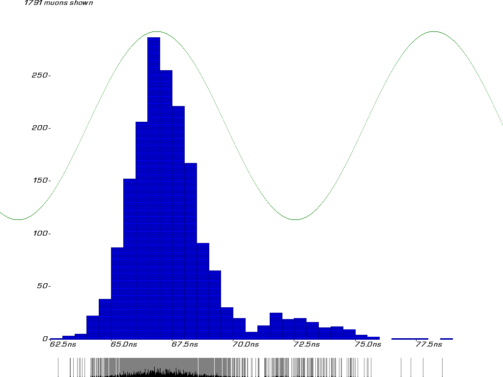
The design is such that muons emitted directly down the solenoid channel with energies in range 120-270 MeV are meant to take an equal amount of time to get to the end of the bends. This means that they are re-bunched longitudinally at that point, ready to be accepted into the third component of the design, an 88MHz linear accelerator (not yet simulated).
These components constitute a muon front end for the Neutrino Factory, with bunched muons leaving the system with a mean kinetic energy of 400MeV. Other front end designs use different combinations of techniques to achieve the same output, for instance by using muon 'cooling' or several stages of linac acceleration.